Forecast Accuracy Improvement for Ecommerce
The most common advice for improving forecast accuracy is to add more data and use a more advanced model. That's often the wrong starting point. A cleaner error score won't help a Shopify buyer who still runs out of a profitable SKU while holding excess stock in the wrong variants.
Start with the purchase decision, measure the direction of your mistakes, and make every new signal earn its place. Live cart behavior can help you anticipate demand, but only when it improves a forecast made with information that was available at the time.
Table of Contents
- Which Forecast Metrics to Track First
- Clean History and Add Live Cart Signals
- Correct Bias Then Combine Models
- Reconcile Store Category and SKU Forecasts
- Validate Cadence and Fix Forecast Drift
- Put Live Cart Data Into Next Week's Forecast
<a id="which-forecast-metrics-to-track-first"></a>
Which Forecast Metrics to Track First
Choose the metric around the decision: reorder quantity, safety stock, staffing, or cart-recovery priority. Those decisions don't carry the same cost of error, so they shouldn't automatically share a score.
Forecast metrics by demand pattern and decision
| Metric | Use when | Breaks when | Decision it supports |
|---|---|---|---|
| MAPE | Stable weekly demand with few zeros | Near-zero or intermittent SKUs | Comparing similar series |
| sMAPE | Stable series where M-competition-style method comparison is needed | Zero-heavy weeks | Choosing a method against a naive benchmark |
| MAE | A few large unit misses drive cost | Series of very different scale | Reorder quantity in units |
| RMSE | Large misses should dominate the score | Outliers or mixed scales distort comparisons | Revenue and high-cost misses |
| MASE | Intermittent or lumpy SKUs | Stakeholders want a raw percent; a flat training series can also make scaling undefined | Method choice versus a seasonal-naive baseline |
| Signed mean error | You must see over- versus under-forecasting | Used alone as an accuracy score | Safety stock and service level |
| WAPE | Volume varies inside one series | All-zero series | Volume-weighted accuracy for the buy |
Say a hero product has a better MAPE than a slow mover, but the hero repeatedly sells out before replenishment arrives. The slow mover never stocks out, yet leaves cash sitting on the shelf. Neither percentage tells the buyer which purchase order to change.
That distinction matters for intermittent demand. A benchmark covering 38 forecasting methods found that service performance was more closely associated with the direction of cumulative forecast bias, particularly systematic overprediction during zero-demand periods, than with point accuracy alone.
<a id="separate-error-size-from-error-direction"></a>
Separate error size from error direction
Define signed error consistently as forecast minus actual. Positive mean error means overforecasting; negative mean error means underforecasting. Absolute-error metrics remove that direction, which is useful for measuring miss size but insufficient for diagnosing inventory consequences.
Track cumulative signed error as well as average bias. Alternating misses can cancel over a reporting period, while a persistent run of underforecasting can exhaust stock before the next delivery.
MAPE gives small-volume periods considerable influence because each period has its own denominator. WAPE pools absolute errors against total actual volume, making it more useful for assessing a buy within a series whose weekly volume changes. It can still conceal individual SKU problems when you aggregate a whole category.
Practical rule: A lower error score is a candidate improvement, not permission to increase or reduce the purchase order.
<a id="lock-the-review-scorecard"></a>
Lock the review scorecard
Before changing a model, agree on the following:
- Primary error metric: Choose the measure that fits the demand pattern and evaluation horizon.
- Signed bias: Keep both the average direction and cumulative path visible.
- Business outcome: Select stockout rate, overstock units, lost margin, service level, or working-capital impact.
Report MAE or RMSE beside percentage metrics, so buyers can see the miss in units or revenue. Define the business metric precisely too: a stockout measured by unavailable SKU-days isn't interchangeable with an order-fill service measure.
Don't reduce safety stock just because point error fell. Test the forecast with the replenishment policy, supplier constraints, and service target that the buyer will use.
<a id="clean-history-and-add-live-cart-signals"></a>
Clean History and Add Live Cart Signals
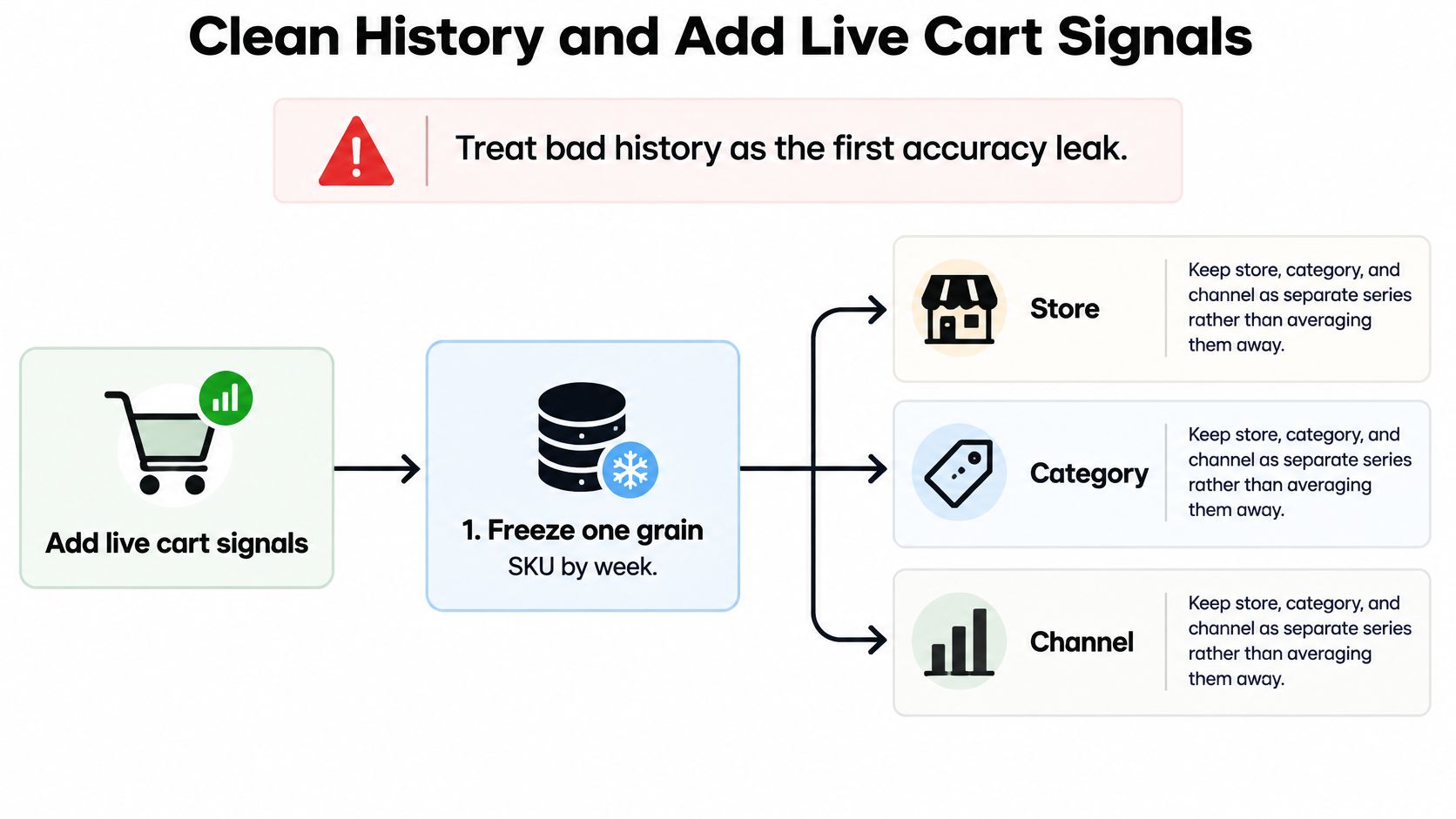
Treat bad history as the first accuracy leak. A model trained on unavailable products, unmarked promotions, and mixed wholesale orders can reproduce those distortions with impressive consistency.
Build a repeatable preparation routine before adding features. A shared data preparation checklist helps the analyst and buyer work from the same definitions rather than maintaining competing spreadsheets.
<a id="build-an-auditable-weekly-table"></a>
Build an auditable weekly table
-
Freeze one grain. Use SKU by week for the purchasing table, with
sku_idandweek_startas the key. Maintain store, category, and channel series separately; don't average them into a number that no longer represents a buyable item. -
Flag stock availability. Keep
in_stock_days,stockout_flag, and observed units sold. A zero recorded while unavailable isn't evidence of zero demand. Impute only periods you can substantiate, preserve the original sales value, and label the replacement so another planner can audit it. -
Date commercial events. Store promotion start and end dates, selling price, discount status, and campaign identifiers. Distinguish planned events from realized campaign performance. Don't let an exceptional discount become the expected full-price baseline.
-
Separate customer and order types. Add new-versus-returning status and DTC-versus-B2B or wholesale classification. Keep identifiable company orders available for separate modeling. A replenishment order from a wholesale account shouldn't reset the expected retail run rate.
-
Attach behavioral counts. Join sessions, product-page views, product searches, add-to-cart events, removals, and checkout starts where attribution is available. Retain device and UTM source as segment fields. Don't distribute an ambiguous search across every SKU that could match it.
-
Lag features to the decision date. Create fields such as
prior_period_cart_addsand recordfeature_available_at. If purchasing happens before the forecast week begins, that week's eventual carts cannot be inputs. Match the lag to the supplier lead time and planning horizon, not whichever lag produces the prettiest fit. -
Freeze the export routine. Export the activity feed to CSV on a fixed weekday and join it to the same sheet or warehouse table the model already reads. Save the export timestamp, timezone, and forecast cutoff. Check duplicate keys and unmatched SKU identifiers before fitting anything.
<a id="keep-intent-separate-from-completed-demand"></a>
Keep intent separate from completed demand
An add-to-cart event isn't an order. A shopper can add several variants, remove most of them, and return later through a different device.
Store removal rate beside add-to-cart rate, with explicit denominators. Separate event counts from unique carts where possible; repeated additions within a cart shouldn't automatically count as independent buyers.
A jump in product views accompanied by removals deserves a merchandising check before a larger purchase. Price, shipping charges, unavailable variants, or delivery promises may be preventing conversion.
The model's approved input table should contain the SKU key, week, observed sales, availability flags, event flags, customer segment, lagged behavior, and availability timestamps. Keep future realized orders, future traffic, and post-cutoff cart activity outside that table.
<a id="correct-bias-then-combine-models"></a>
Correct Bias Then Combine Models
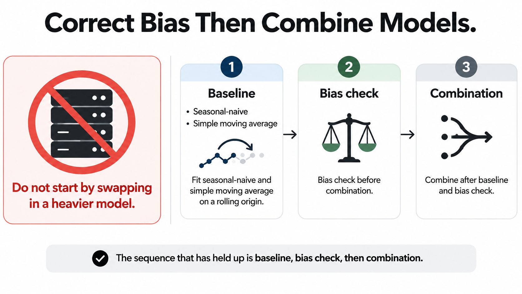
Fit a seasonal-naive forecast before considering a heavier model. For a suitable seasonal series, it repeats the corresponding historical seasonal observation. Fit a simple moving average alongside it so you can distinguish genuine seasonality from a recent level change.
Run both through rolling-origin evaluation: train on the past, forecast the required horizon, advance the cutoff, and repeat. Save each forecast as issued rather than overwriting it when actual orders arrive.
<a id="correct-a-persistent-miss-before-adding-complexity"></a>
Correct a persistent miss before adding complexity
The distinction between descriptive analytics and predictive analytics becomes practical here. Describing last week's miss is diagnosis; predicting the next period requires a correction that works beyond the observations used to estimate it.
Use a validation slice that is separate from the final evaluation period:
- Locate the bias: Break signed error down by device, traffic source, customer type, SKU velocity, and horizon where sample sizes support the split.
- Check persistence: Look for repeated directional misses rather than correcting a single unusual week.
- Apply the adjustment: Subtract estimated signed bias from the base forecast, then enforce sensible nonnegative demand constraints.
- Refresh deliberately: Reassess after a major campaign or a material change in assortment, rather than carrying a stale correction indefinitely.
In temporal-hierarchy forecasting work, bias adjustment delivered about 1.5% average improvement, while combining forecasts across methods and aggregation levels produced roughly 2% average improvement. Those are findings from that evaluation, not promised lifts for a Shopify catalog.
A small correction can be preferable to a complicated replacement if it remains stable and easy to explain. Don't create fine-grained corrections for segments with too little evidence to distinguish systematic error from noise.
<a id="combine-forecasts-that-make-different-mistakes"></a>
Combine forecasts that make different mistakes
Generate another forecast from a different family. ETS or ARIMA can represent weekly sales patterns; a lightweight regression or other feature-based model can test whether lagged cart behavior adds information.
Use validation performance to set combination weights, with safeguards against giving all the weight to a model that won during an unusual campaign. If several models make nearly identical errors, adding them together offers little diversification.
The M4 Competition findings showed that 12 of the 17 most accurate methods were combinations, and the best method improved sMAPE against Naïve 2 by 16.2%. The leading approach mixed statistical and machine-learning elements.
Keep the naive forecast in production comparison until the replacement wins repeatedly at the horizon buyers use.
Don't automatically reject future promotion plans: a calendar approved before the forecast cutoff is usable. Reject realized future traffic, final campaign results, and promotion details reconstructed afterward. Historical backtests need the information available then, not today's corrected version of the past.
<a id="reconcile-store-category-and-sku-forecasts"></a>
Reconcile Store Category and SKU Forecasts
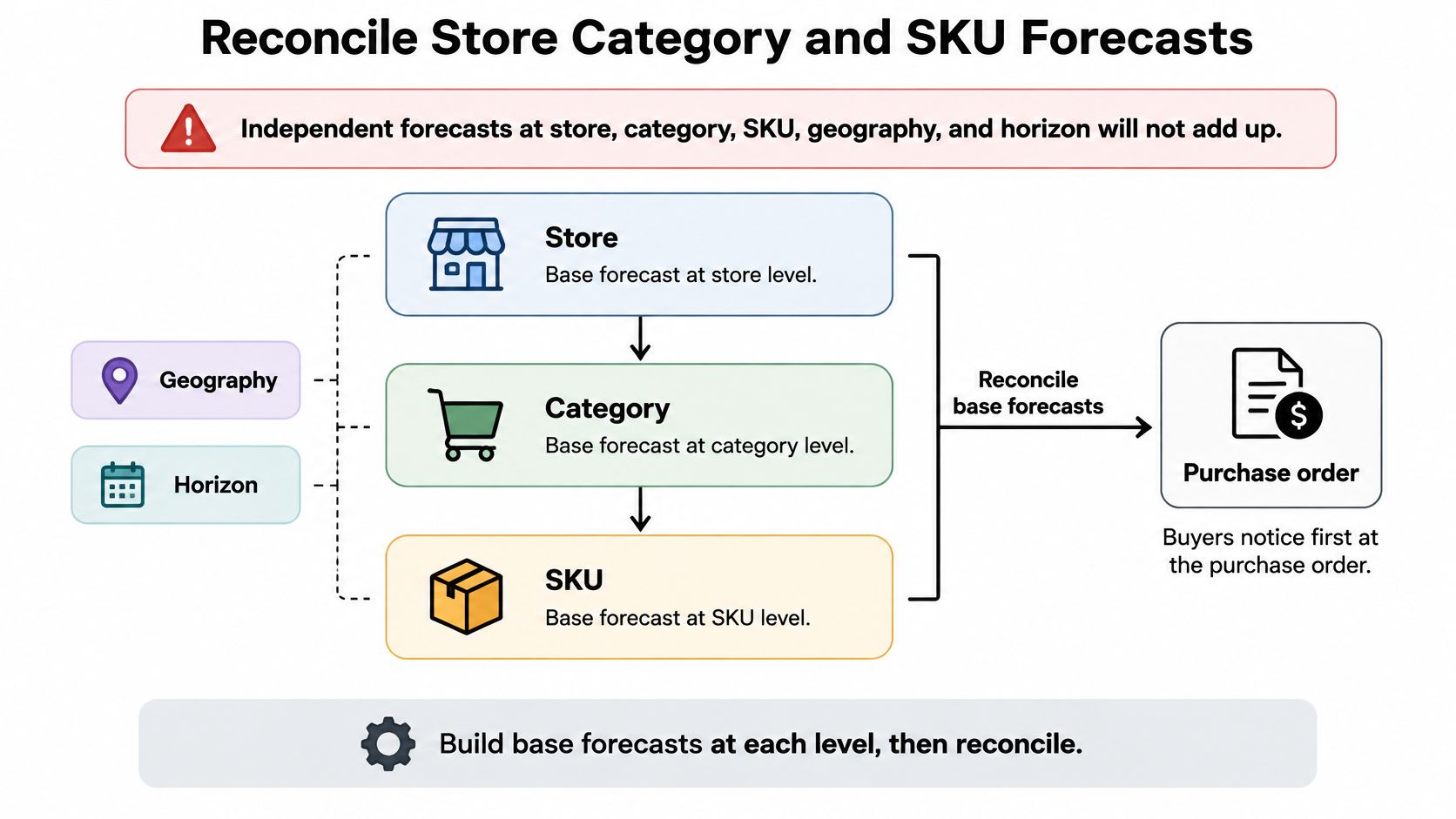
Independent forecasts won't necessarily agree. The store forecast may imply a larger buy than the category forecasts, while SKU forecasts imply something else again. Buyers encounter that conflict when deciding which purchase-order lines to approve.
Hierarchical reconciliation makes the planning numbers coherent. Build base forecasts at meaningful levels, then adjust them together so SKU quantities sum to category totals and categories sum to the store total.
<a id="make-the-purchase-order-add-up"></a>
Make the purchase order add up
In a Portuguese retail study using 1,751 series, Minimum Trace Shrinkage generally improved ARIMA accuracy, with complete-hierarchy gains of approximately 1.7% to 3.7%. The gains tended to increase at longer horizons.
Treat that result as support for testing reconciliation, not a reason to force it onto every product. Start with a stable hierarchy and explicit membership rules:
- Store and category: Assign each SKU to a purchasing category without double-counting products that appear in several merchandising collections.
- SKU and geography: Keep location-specific demand where fulfillment or buying decisions differ.
- Company demand: Give material B2B accounts a separate branch when their purchasing behavior warrants it.
- Time aggregation: Make weekly and longer-period plans consistent where they represent the same demand and calendar boundaries.
Minimum Trace approaches use relationships among forecast errors to distribute adjustments. In practice, that requires a trustworthy forecast-error history. Sparse or newly introduced series need more caution than established products.
Avoid solving the disagreement by multiplying every SKU by the same store-level factor without testing it. That can preserve a grand total while distorting the mix buyers need.
<a id="constrain-the-funnel-without-inventing-identities"></a>
Constrain the funnel without inventing identities
Behavioral forecasts require a related but different check. Sessions, product views, cart additions, removals, and completed orders are not additive children of the same total. A shopper can generate repeated events, and an order can contain several units.
Define the units before applying funnel constraints. Unique carts, unique shoppers, event counts, order counts, and units sold shouldn't be used interchangeably.
Where definitions support it, test conversion relationships and plausible bounds between stages. If the forecast implies completed orders inconsistent with the expected converting-cart population, inspect attribution and model assumptions. Don't force product views to sum to sessions just to make a dashboard look tidy.
For a launch, use comparable category behavior as a prior, not as proof of its individual demand. Keep uncertainty visible while product-specific evidence develops.
Publish one operational number per SKU per week, together with the category total and an exception register. If an unreconciled SKU forecast wins on a predefined segment, retain that result and recompute the parent total from the chosen children. Keep the unreconciled model when it wins, but never leave buyers with conflicting totals.
<a id="validate-cadence-and-fix-forecast-drift"></a>
Validate Cadence and Fix Forecast Drift
Set a weekly review rhythm with a frozen forecast cutoff. Score the forecast that was issued, investigate exceptions, and distinguish refreshing inputs from refitting the entire model.
I'd refresh the operational forecast on a fixed weekday and change weights on a slower, scheduled cadence unless a material event justifies intervention. For longer supplier commitments, review whether the remaining buy is still appropriate rather than retraining daily on noise.
<a id="diagnose-the-failure-before-changing-the-model"></a>
Diagnose the failure before changing the model
Forecast failures and the fix to ship
| What you see | Usual cause | Fix before the next cycle |
|---|---|---|
| MAPE blows up on a sparse SKU | Zeros and lumpy orders | Score that series with MASE and bias, not MAPE |
| Backtest looks strong, live week fails | Possible future promotion or traffic leakage | Drop features not known at forecast time and rerun the rolling origin |
| Views surge but orders do not | Browsing without conversion | Pair add-to-cart with removal rate, price, and shipping before raising demand |
| Bias flips after a sale | Campaign-regime change or a correction fitted on the evaluation window | Re-estimate bias only on the validation slice and inspect the event boundary |
| Category buy no longer matches SKUs | Inconsistent overrides or reconciliation that hurt a level | Retain the winning unreconciled segment and rebuild the parent total |
| New launch has almost no orders | History too short to trust | Use category shape as a prior and lagged page, search, and cart signals |
These are investigation routes, not automatic diagnoses. A live miss can also reflect a supplier failure, an unexpected promotion, or a tracking change. A bias reversal alone doesn't prove leakage.
Keep charts for error relative to the seasonal-naive forecast, cumulative signed bias, and stockout or overstock outcomes on margin-critical products. Compare like-for-like horizons and cohorts so an assortment change doesn't masquerade as model deterioration.
Deployment gate: Don't accept an aggregate win that makes the commercially important segment worse.
<a id="handle-sparse-demand-as-a-separate-problem"></a>
Handle sparse demand as a separate problem
Classify intermittent products before choosing a fix. Repeated zero-demand periods, occasional wholesale orders, and a new launch with no history are different forecasting problems.
Hyndman's guidance on intermittent-demand accuracy supports MASE as a scale-free alternative for comparing methods across series. Use a clearly documented naive scaling rule, seasonal where appropriate, and check that the training history produces a meaningful denominator.
For a new SKU, historical scale-based metrics may not yet be available. Assess comparable launch cohorts, report unit errors once observations accumulate, and avoid presenting a fragile percentage as a reliable benchmark.
Behavioral indicators can help fill the information gap, but inspect their meaning. Company activity and assisted-sales quotes may be more useful for a wholesale item than broad browsing volume. Product interest without checkout progress may call for a shipping or pricing intervention rather than more stock.
More history isn't always the answer. Old observations from a discontinued price position, different pack size, or obsolete acquisition channel can make the current forecast worse. Fix the demand classification and uncertainty estimate before increasing model complexity.
<a id="put-live-cart-data-into-next-weeks-forecast"></a>
Put Live Cart Data Into Next Week's Forecast
Run a bounded pilot rather than switching the catalog at once. Include hero products, intermittent sellers, and recent launches, and define the keep-or-drop rule before viewing the results.
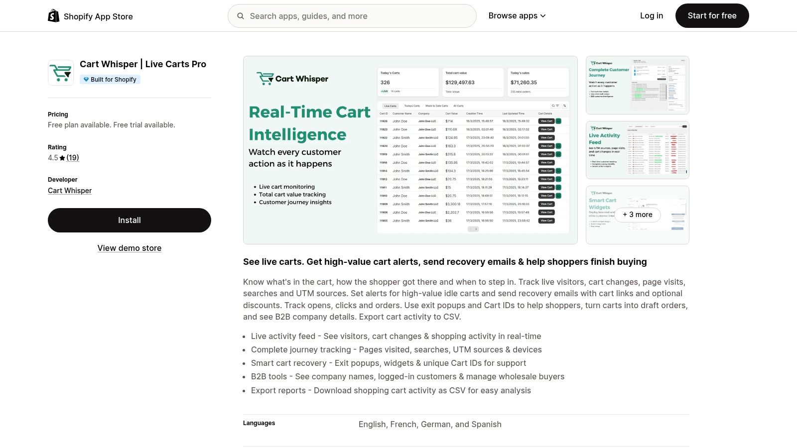
Use Cart Whisper | Live View Pro as the live activity export, not as a demand-forecasting engine. Complete journey tracking shows pages visited, searches, UTM sources, and devices, while activity can be exported as CSV for analysis in Excel or Google Sheets. Logged-in company details and cart history also help analysts distinguish wholesale intent from retail browsing.
<a id="give-the-pilot-a-purchase-decision"></a>
Give the pilot a purchase decision
The useful application of real-time ecommerce analytics is a specific intervention, not a faster-moving dashboard. Join the exported behavior to the weekly SKU table, then compare a forecast with those features against an otherwise comparable forecast without them.
Keep the operational comparison fair:
- Same information cutoff: Both forecasts must use only information available when the buyer commits.
- Same evaluation periods: Compare identical SKUs, horizons, and availability conditions.
- Same inventory policy: Hold replenishment rules constant while testing the forecast change.
- Named owners: Assign the scorecard to an analyst and the purchase decision to a buyer.
A short pilot can establish whether the export, joins, and forecast snapshots work. It can't establish long-horizon forecasting value before the relevant outcomes exist. Continue evaluation until repeated rolling windows provide enough evidence for the decision.
<a id="keep-only-signals-that-change-the-right-outcome"></a>
Keep only signals that change the right outcome
Retain cart features where the primary error measure and the chosen business outcome improve consistently. If they reduce percentage error but increase hero-product shortages or excess units, reject that deployment for the affected segment.
For B2B demand, review company-level activity before treating a large cart as recurring demand. A stalled wholesale cart may need a draft order, invoice, or assisted follow-up. Resolving that transaction is different from increasing the expected retail run rate.
Document accepted features, rejected features, and the reason for each decision. That record lets the next planner distinguish an intentional exclusion from a broken data join.
Forecast accuracy improvement is successful when the buyer makes a better commitment. The final test is whether the signal changes what you buy, when you buy it, or how you assist the shopper, without creating a more expensive problem elsewhere.
Cart Whisper | Live View Pro gives your team visibility into live shopper journeys and cart activity, with CSV exports you can test alongside weekly SKU forecasts. Visit Cart Whisper | Live View Pro to evaluate the activity feed, build a lagged-behavior pilot, and keep only the signals that improve purchasing or recovery decisions.